Optimizing Memory Bound Kernel to Speed of Light

Making memory bound kernel reach speed of light because why not !!

Memory-bound kernels are the worst - no flops, no major compute, just transferring data from one location in HBM to another. Hence optimizing them becomes extremely important.

In this blog post we will be optimizing 2 operations used majorly in LLMs -

• Embedding Kernel

• RMS Normalization

Why the above 2 operations and why not activation functions too ?? I mean, if you see ReLU activation function, its simply f(x) = max(x,0) → totally memory bound.

Well, activation functions are used after a linear layer, and they can be fused easily.

How ??

In 2 ways :

1. Using torch.compile(). PyTorch has Triton kernels with a fused linear layer and activation function. Eg: triton_poi_fused_addmm_relu_0

2. Using CUTLASS - its GEMM operation exposes epilogue API which can be used to fuse activation functions.

Now what exactly is a memory-bound kernel, and how to determine whether a kernel is memory-bound or compute-bound?

Arithmetic Intensity

Arithmetic Intensity is the ratio of the number of operations to the number of memory operations.

Formula :
AI = (Floating Point Operations) / (Memory Traffic (Bytes))

If AI is high, then the kernel is compute-bound.

If AI is low, then the kernel is memory-bound.

Simple!

Memory-bound kernels are the kernels bounded by the memory bandwidth of your GPUs.

So the very first obvious step is to find the memory bandwidth of your GPUs.

You can check your GPU info here :

https://en.wikipedia.org/wiki/List_of_Nvidia_graphics_processing_units

I have RTX 3050 4Gb 70W (GPU Poor), so for me:

• Memory Bandwidth: 168 GB/s

• half and single precision : Base clock = 4.802 TFLOPS | Boost Clock = 6.774

• Tensor cores: 30.1 | Sparse = 60.2

Now, here is a catch: the memory bandwidth specifier is of your HBM, so if you write a kernel that only uses HBM, then the memory bandwidth will be capped at that amount. However, most of the time, kernels will also utilize L1 and L2 caches. So don’t be fooled by the memory bandwidth specifier as the speed of light.

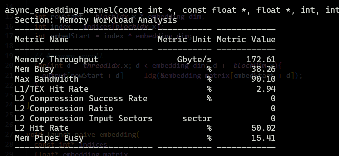
A better way to profile is to use NCU (NVIDIA Nsight Compute) to profile your kernel and get the Memory workload analysis.

Here is how you can do that

ncu --section MemoryWorkloadAnalysis -c 5 <binary>

It will give you:

• Memory Throughput (Gb/s)

• Max Bandwidth (%)

• L1/Tex Hit Rate (%)

• L2 Hit Rate (%)

• Mem pipes Busy (%)

Embedding Kernel

An embedding kernel is the kernel that converts the token IDs to embeddings.

Formula :

def embedding_kernel(token_ids, embedding_table):
    return embedding_table[token_ids]

Here token_ids is of shape (batch_size, seq_len) and embedding_table is of shape (vocab_size, embedding_dim)

So total bytes = (bytes to load + bytes to store) = seq_len * batch_size + seq_len * batch_size * embedding_dim

Hence:

Arithmetic Intensity = 0 / (seq_len * batch_size(1 + embedding_dim)) = 0

Memory Bound!!

Optimization 1: Ensuring Coalesced Access

This is the single most important optimization in memory-bound kernels. If you do this right, you can just close your IDE and have a good night's sleep. Further optimizations are only for the sake of bragging rights.

What is coalesced access?

Modern GPUs move data in cache-line-sized chunk sizes, which is typically 128 bytes, from L2 cache/DRAM. Coalesced access means we ensure all the 128 bytes of data that are accessed in one transaction are relevant to our operations.

Example :

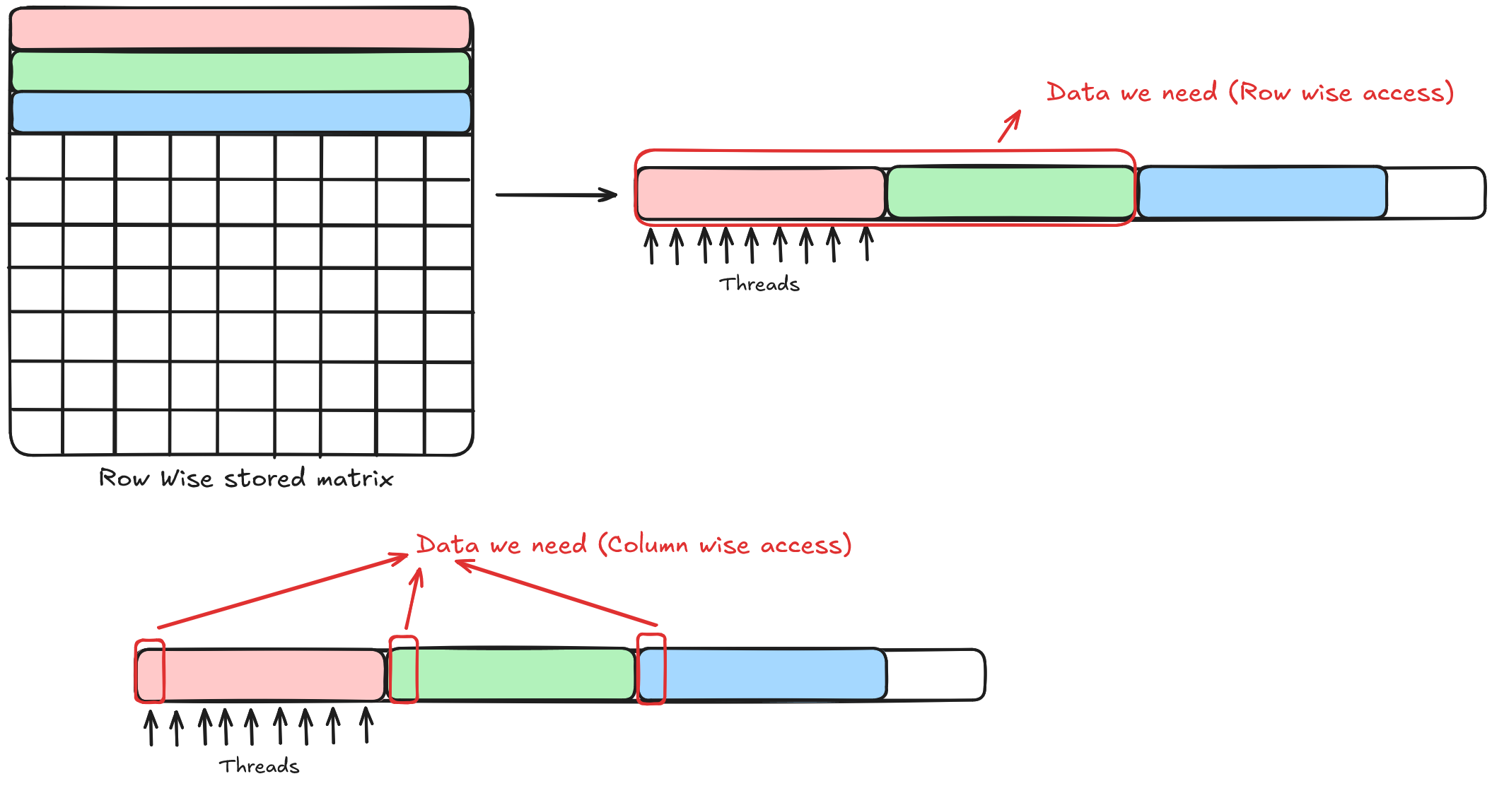
As we can see in the diagram above, we have a row-wise matrix. Now, if we access elements in row-wise fashion, considering the data type as fp32, which means 32 threads or 1 warp will be accessing 32 elements at once (128 bytes / 4 bytes = 32 fp32 elements).

So one transaction will be accesing data from Matrix[0][0] to Matrix[0][31] and the data we want is Matrix[0][0] to Matrix[0][31] → perfectly aligned.

Now in the case of column wise matrix, we will be accessing data from Matrix[0][0] to Matrix[31][0] and the data we want is Matrix[0][0] to Matrix[0][31] → so only the element Matrix[0][0] is relevant to us and rest 31 elements are just noise. Which means to access 32 elements, we need 32 transactions in column-wise access, but only 1 transaction in row-wise access.

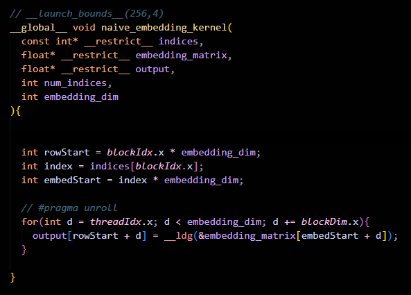
Luckily, in our case, in embedding kernel it’s easy to ensure coalesced access.

Here is the code:

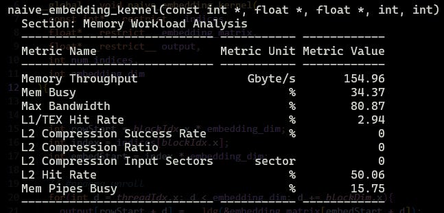
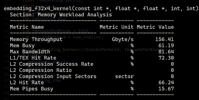
Here is what we got for our naive embedding kernel:

Optimization 2: Vectorized Load and Store

This, combined with coalesced access, should be your holy grail for memory-bound kernels.

There are two distinct vectorized load/store implementations worth highlighting before we analyze the source of the performance gains:

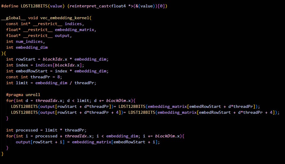
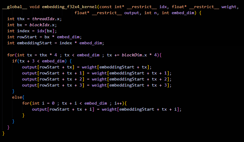
1) Reinterpret Cast to float4: This approach uses reinterpret_cast to convert float* pointers to float4* pointers, treating groups of four single-precision values as a single vector unit. Since this cast occurs at compile time, it adds no runtime overhead. The memory operations then utilize these vector types directly.

Here is the code for that:

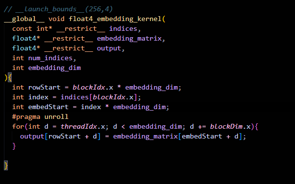
2) Using float4 Pointer Parameters: Here, the kernel itself accepts input and output pointers explicitly typed as float4*. This design makes the vectorized intention clear at the interface level, avoiding the need for internal pointer reinterpretation.

Again the code for this too:

Let’s see the results:

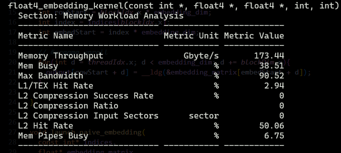
Clearly, conversion on the fly is faster, but why ??

The reason is in the line :

LDST128BITS(output[...]) = LDST128BITS(embedding_matrix[...]);
LDST128BITS(output[... + 4]) = LDST128BITS(embedding_matrix[... + 4]);

By manually unrolling two float4 loads/stores back-to-back, we are increasing Instruction Level Parallelism.

The CUDA compiler and the GPU hardware scheduler are much better at hiding latency when they see multiple independent 128-bit loads issued in a row. It can fire off the first load, then the second, and then wait for both.

Another reason is quite visible to us in the profiler output - creating spatial locality.

When we load float4, the GPU loads an entire 128-byte cache line into L1 cache, so our next float4 is already in L1 cache, and we can just load it from there.

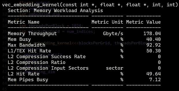
Now, let’s compare coalesced access vs vectorized access

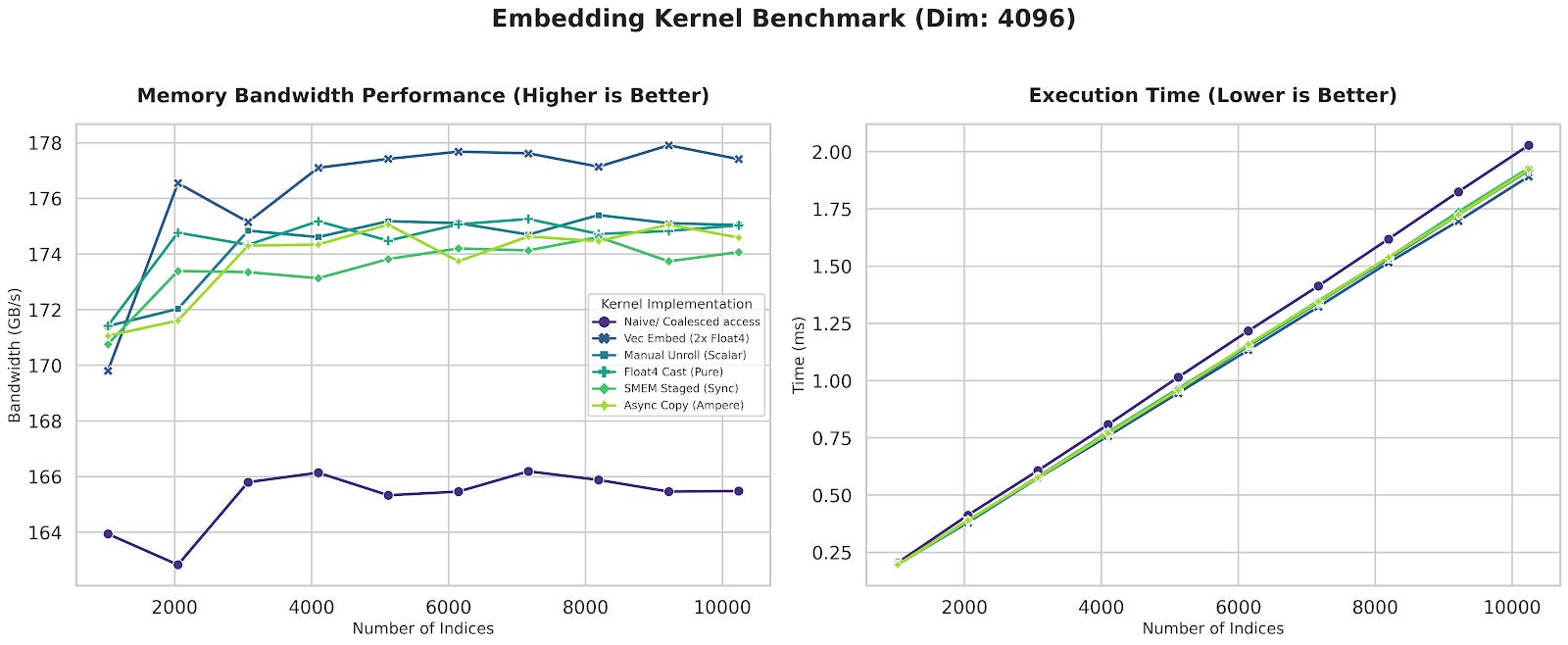
We got a boost from 154.96 Gb/s to 178.04 Gb/s.

Why is that? I mean, to the naked eye, there should be no difference, right ? Because the bandwidth of memory is 128 bytes, so I can either access 32 different elements of 4 bytes each (fp32) or 8 elements of 16 bytes each (float4) - should not make any difference right?

Well, the main optimization of vectorized load and stores is from Instructions per Clock (IPC). Lemme explain :

Every instruction in CUDA has a cost. Even if your memory is coalesced, the Warp Scheduler has to physically “issue” the load instruction.

Naive Kernel: To move 128 bytes (32 floats), the warp scheduler must issue 32 individual 4-byte load instructions (one per thread).

Vectorized Kernel: To move the same 128 bytes, the scheduler issues 8 vectorized 16-byte load instructions (LDG.E.128).

We are reducing the workload of the Warp Scheduler by 4x

On modern architectures like Ampere, Hopper, or Blackwell, the scheduler can become the bottleneck if you’re spamming it with thousands of tiny 32-bit requests.

On top of this, we are increasing the Instruction Level Parallelism (ILP) as well as spatial locality, as explained above

Degradation 1: Loop unrolling

This is the optimization we normally do in memory-bound kernels to increase the work done by each thread as well as register pressure.

Here is the code as well as the result to do so:

Wait what? No perf gains? why?

The reason is obvious: we don’t have anything to compute to hide the memory latency. On top of it, the memory access is not exactly coalesced.

Thread 0 is accessing element {0,1,2,3} and Thread 1 is accessing element {4,5,6,7}, and so on, but each of them is accessing only the first element from DRAM and others from L1 cache, like Thread 0 accesses 0 from DRAM and the rest of the elements move to L1 cache. That’s why we see a high use of L1 cache but no increment in performance

Degradation 2: Using Shared Memory

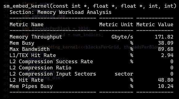
Here is a quick code snippet and the results, and then we will talk about the reason for the degradation.

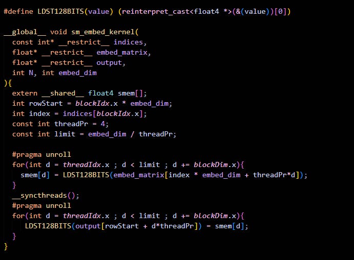
One might assume “Shared Memory is fast and it’s closer to DRAM too, so I should always use it,” but that’s the trap.

When we use shared memory, we are effectively introducing a middleman that charges a tax and provides no value (sounds like our government).

In normal coalesced access or vectorized access, the flow is:
HBM —load→ Registers —store→ HBM (Happy life)

But in the case of shared memory, the flow is:
HBM —load→ Registers —store→ Shared Memory —load→ Registers —store→ HBM (Sad life)

On top of this comes the synchronization barrier.

In our SM kernel, we have __syncthreads() , which basically forces every single warp in the block to wait until the slowest warp finishes writing to SMEM.

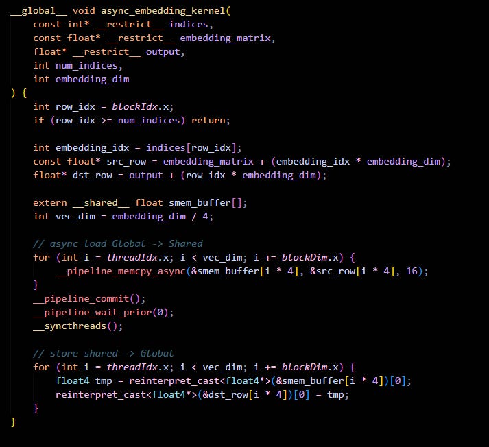
Degradation 3: Using Asynchronous Memory Copy

But wait, I see the main reason for degradation - it’s using a register between shared memory right?! Let me use async memcpy to copy data from HBM to SMEM, bypassing the registers. Problem solved, hurray !!!!
Here lemme code it up quick

Finally, let’s just our results

Wait what !! No perf gains? I even did vectorized load and store !! What happened ?!

Here is what happened

First of all, it only bypasses Registers on the LOAD. cp.async moves data from Global Memory → Shared Memory, but it does NOT help the STORE.

So effectivly we are doing HBM —load→ Shared Memory —load→ Registers —store→ HBM

Second, if you see in the profiler output ,we are getting L1 Hit Rate: 2.94% cp.async explicitly bypasses the L1 Data Cache to write directly to Shared Memory banks. We threw away the “free speed” of the L1 cache. Every single byte had to go to L2 or DRAM.

Basically,

Vec Embed: “Hey Memory, give me data.” -> (Cache says: “Here it is!”) -> “Okay, writing it back.”

Async Embed: “Hey Async Engine, set up a pipeline. Commit this group. Wait for this group. Bypass the cache. Put it in Shared Memory. Now read it back from Shared Memory. Now write it.” -> Slower.

Async is designed to hide memory latency by allowing the GPU to crunch numbers while data travels from HBM to Shared Memory. In an embedding lookup, we are purely limited by how fast we can pull data from HBM. cp.async introduces overhead: pipeline management, synchronization (cp.async.wait_all), and banking conflicts in Shared Memory.

Final Benchmark

Here is a comprehensive comparison of all the discussed methods

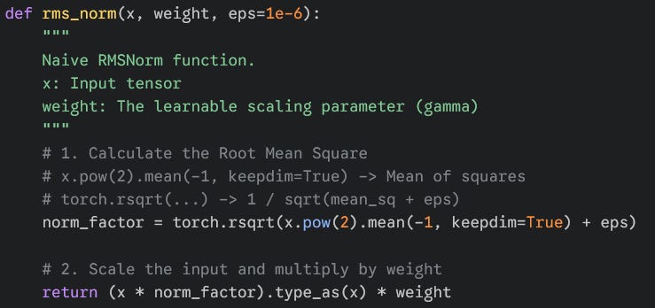
RMSNorm Kernel

RMSNorm is the most used normalization method in LLMs. It is a simple operation that normalizes the input by the square root of the mean of the square of the input.

So for a single vector of dimension D:

Total Flops = 4d (Square + add + normalize and scale)

Total Bytes (fp16 or bf16) = 2d (load) + 2d (weight) + 2d (store)

Arithmetic intensity = Flops / Bytes = 4d / 6d = 2/3 = 0.667

Hence Memory Bound

Here is a naive implementation of RMSNorm in PyTorch to showcase the operations

Optimization 1: Coalesced access + Shared Memory

The thought process behind this approach is pretty simple.

We have M x N matrix, where M = number of different tensors and N = dimension of each tensor.

Approach

What we can do is allocate one tensor to one block of threads, resulting in M blocks of threads in a grid.

Each thread will be responsible for loading (dimension of tensor) / (threads per block) elements of the tensor.

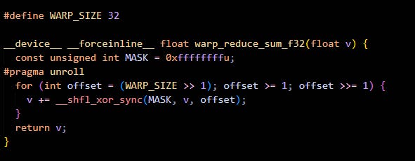
First and foremost, we need the sum of all the elements of the tensor, then compute the Root Mean Square. let’s tackle that first

Sum is a reduction operation, and we can use the warp shuffle instructions to perform it for a warp, the code for which looks like this

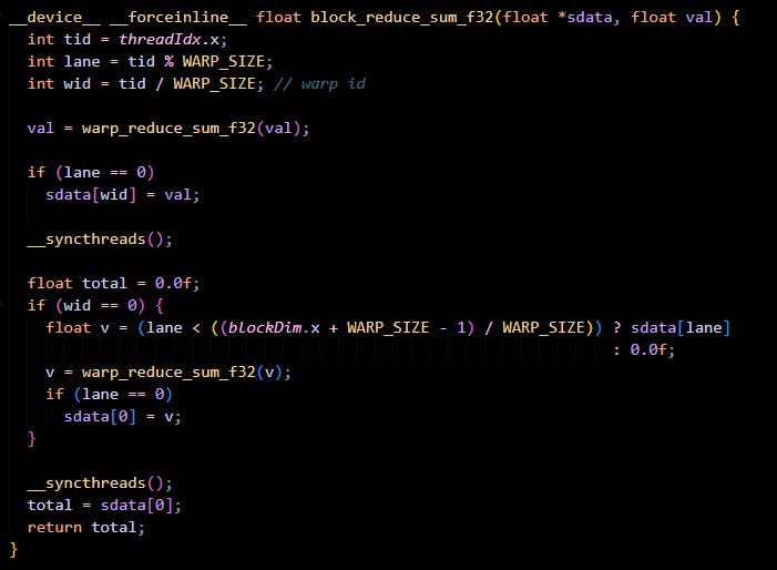
Zooming out from a warp, we get a thread block. We can make a block reduction kernel that uses warp reduction to perform reduction for a block.

The code is pretty simple :

Now that we have the mechanism to get a sum across a block of threads, we just need to make sure that the block contains a partial sum for the whole tensor.

This can be done by something like :

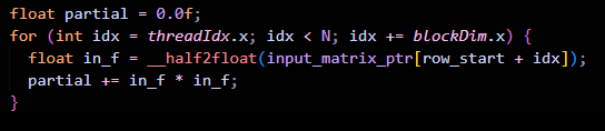
Here , each thread is holding the sum of (dimension of tensor) / (threads per block) elements of the tensor.

Now we can use the block reduction across the sum to get the final sum of the tensor.

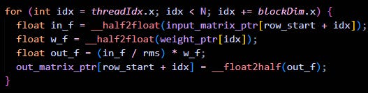
Next step is to compute the Root Mean Square, which is pretty simple :

 float rms = sqrtf((total_sum / N) + eps);

The final step is to apply the RMS and apply weights to each element. Which can be done easily as shown :

Here is the final code for our RMSNorm kernel : [code snippet for rmsnorm kernel]

Now lets profile:

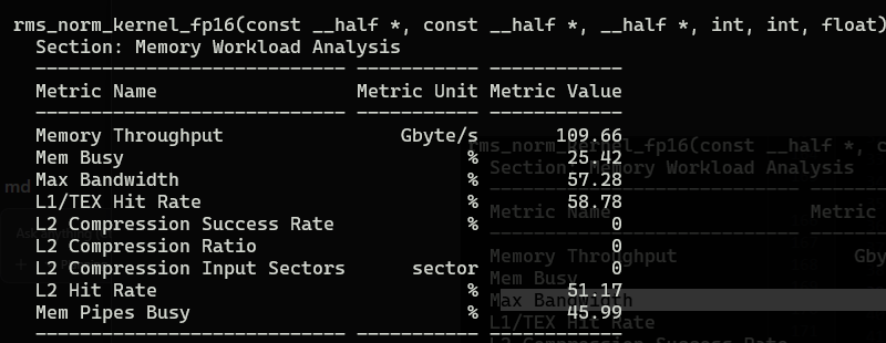
Memory throughput is only 109Gb/s, and bandwidthis only 57.28%

Well, time to use what we learned above - vectorization !!!

Optimization 2 : Vectorization

As explained in-depth above, to saturate the memory bandwidth, we need to perform vectorized load and store.

This time we are dealing with half precision so we will be using half2

#define LD32BITS(value) (reinterpret_cast<const half2 *>(&(value))[0])
#define ST32BITS(addr, value) (reinterpret_cast<half2 *>(&(addr))[0] = (value))

The important thing in dealing with half precision is you should never ever do any kind of arithmetic operations on it, always use __half2float() for converting the half to float and then performing the operations for the sake of preserving the accuracy.

Another optimization is shared memory. If you see, we again have to access all the elements of the tensor from the HBM for applying the normalization and store back - that’s a total of 1 extra global memory access, and here is where shared memory comes into the picture.

What we can do is , while computing the partial sum - we can store the elements in shared memory. So the modified partial sum looks like this :

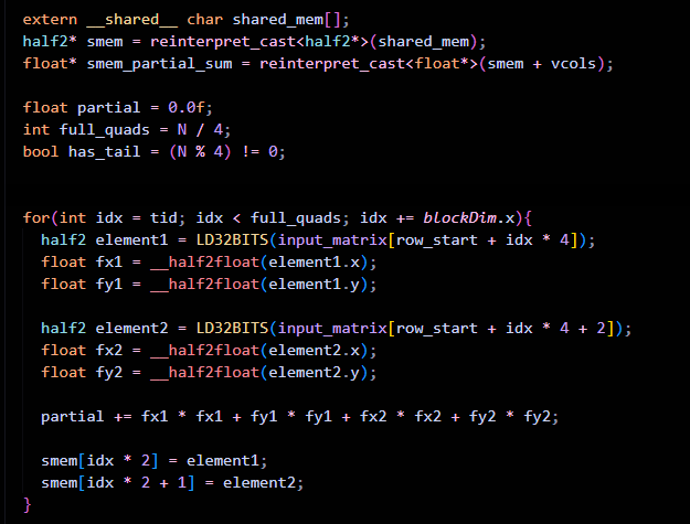
From shared memory, we can fetch the elements, apply RMS, apply weights to each element and finally store back to HBM.

Here is the final code for our RMSNorm kernel :

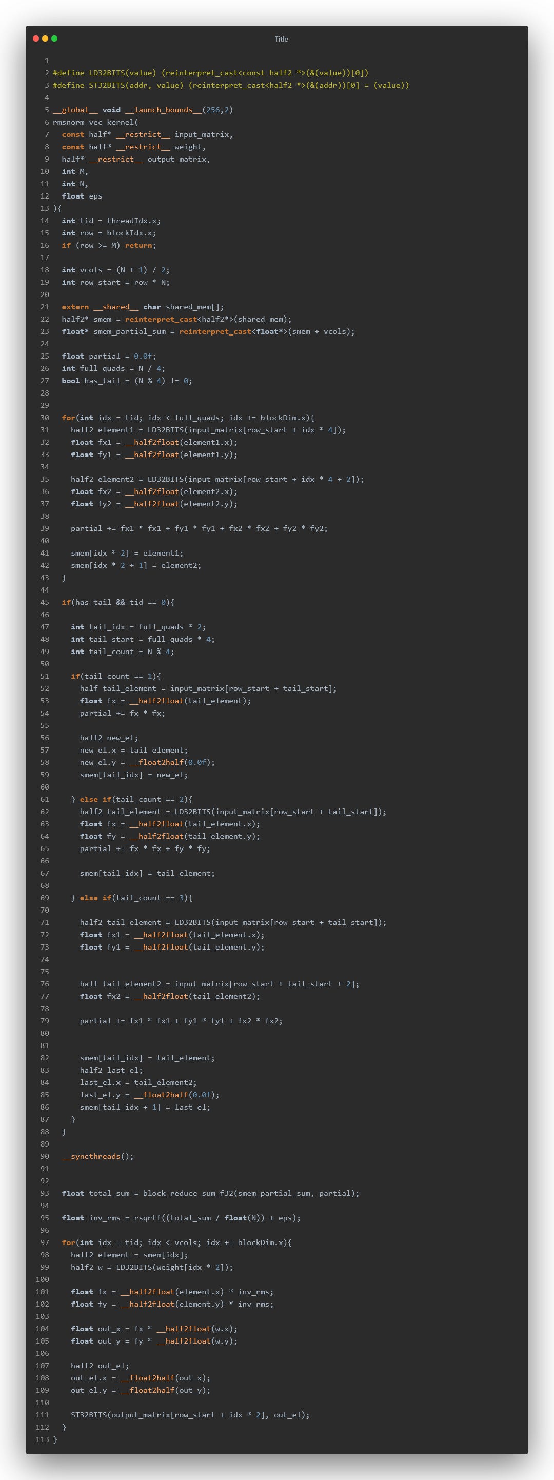
Now let’s profile:

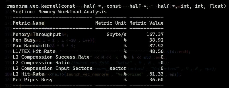
Well 109GB/s to 167GB/s and 57.28% to 87.42% is a pretty good boost

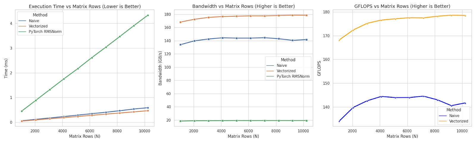
Final Benchmark

Here is a comprehensive comparison between the two + PyTorch’s RMSNorm

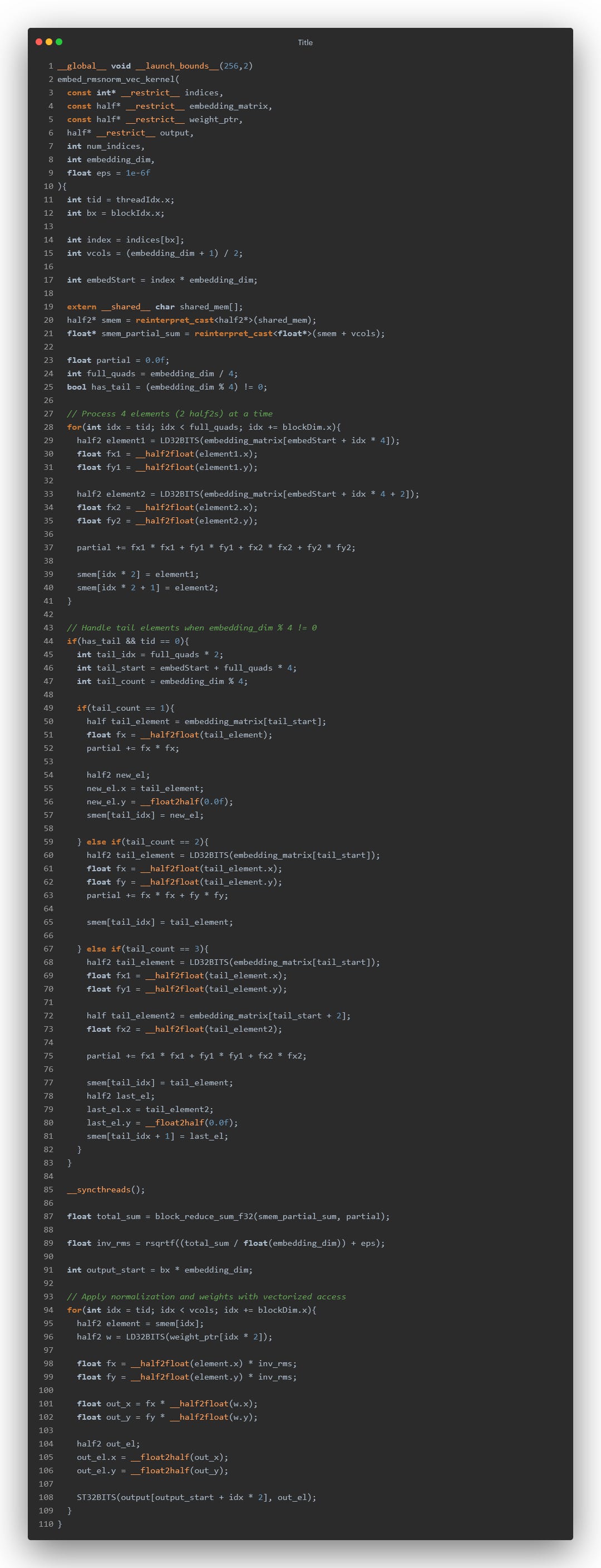
Fused kernel

For memory-bound kernels, the best thing you can do is to fuse the operations.

So its time to fuse the RMSNorm kernel with the embedding kernel.

Now I won’t be going through the entire process of optimization, let’s just directly apply everything we learned - coalesced access, shared memory, vectorization.

The code :

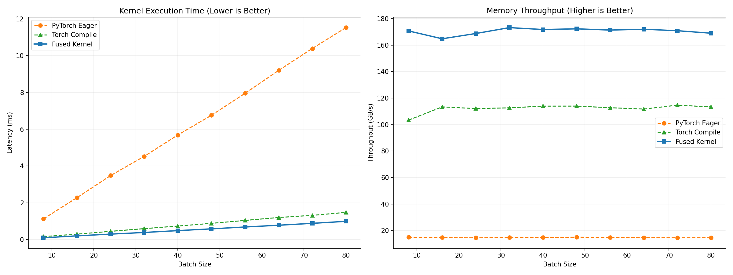
Now we are going to benchmark this against:

1. Naive PyTorch Code

2. torch.compile()

The final result is :

Conclusion

Optimization isn’t about throwing every CUDA feature at the wall.

1) Know your bottleneck: If you are bandwidth-bound, cp.async and loop unrolling won’t save you.

2) Vectorize everything: Increasing the transaction size (fp32 -> float4, half -> half2) is the single highest ROI change you can make.

3) Profile, don’t guess: Naive intuition said “Shared Memory = Fast.” The profiler said “L1 Cache Hit Rate = 2%.” The profiler always wins.